Drawing three-dimensional plot specified by a function f(x,y) in R

Some of the plots described previously in this blog actually give visualizations of functions in two variables. Examples are the quiver and contour plots. Another one is a perspective plot which can be created by calling the appropriately named plotting function persp() of R.

Here is a simple example: f(x,y) = sin(x) + cos(y), whose figure is displayed below:

It can be quite messy to do it from the R console. The solver page provides a fill-in-the-blanks settings page which describe the figure. By way of illustration, here is the R code for the figure above with line numbers. Intermediate output is shown interspersed without a leading ">" prompt. This happens after the summary report for the z values.

0001 > png("tmpZzY7bz.png", width = (6)*72, height = (6)*72)
0002 > f <-function(x, y){sin(x) + cos(y)}
0003 > x <- seq(-10, 10, length.out = 100)
0004 > y <- seq(-10, 10, length.out = 100)
0005 > tridata <- outer(x, y, f)
0006 > z <- tridata
0007 >     summary(as.vector(z))
0008 Min.  1st Qu.   Median     Mean  3rd Qu.     Max.
0009 -1.99900 -0.79430 -0.04088 -0.06207  0.63990  1.99600
0010 >
0011 > z0   <- min(z) - (max(z) - min(z)) / 100
0012 > z    <- rbind(z0, cbind(z0, z, z0), z0)
0013 > x    <- c(min(x) - 1e-10, x, max(x) + 1e-10)
0014 > y    <- c(min(y) - 1e-10, y, max(y) + 1e-10)
0015 > fill <- matrix("green3", nr = nrow(z) - 1, nc = ncol(z) - 1)
0016 > fill[, i2 <- c(1, ncol(fill))] <- "gray"
0017 > fill[i1 <- c(1, nrow(fill)), ] <- "gray"
0018 > fcol <- fill
0019 > fcol[] <- terrain.colors(nrow(fcol))
0020 > fcol   <- fill
0021 > zi <- tridata[-1, -1] + tridata[-1, -ncol(tridata)] + tridata[-nrow(tridata), -1] +tridata[-nrow(tridata), -ncol(trida
0021 a)]
0022 >
0023 > fcol[-i1, -i2] <- topo.colors(20)[cut(zi, quantile(zi, seq(0, 1, len = 20 + 1)), include.lowest = TRUE)]
0024 >
0025 > persp(x, y, 1 * z, theta = 135, phi = 30, col = fcol, scale = FALSE, ltheta=-120,lphi=0,shade = 0.75, border = NA, tic
0025 type = "simple", box = FALSE)
0026 > title(main = "3D Plot", font.main = 4)
0027 > par(bg = "slategray")
0028 >
0029 > graphics.off()
0030 > #img tmpZzY7bz.png

The solver page which generates 3d figures is at /solvers/rplotpage/trid.

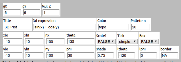
The part of the menu page for the settings of 3d plots is shown here: