Wednesday, August 21, 2013

August 21, 2013: A painful reinstallation and rewrite of our extreme site.

It was working before extremely well with Quixote server. In my desire to upgrade to the latest QP , QPY webserver system, I have wrecked my hard work of so many years. But I know the developers of QP and QPY have a gem of a web server framework. It just occupies a few space in a Linux system. So we start documenting a fresh rewrite of our solvers using QP, QPY.

Here is what we did.

1. Download the installation files.


wget -ct 0 --no-check-certificate https://www.mems-exchange.org/software/DurusWorks/DurusWorks-1.2.tar.gz
wget -ct 0 --no-check-certificate https://www.mems-exchange.org/software/dulcinea/Dulcinea-0.22.tar.gz


2. Install DurusWorks first.

Unpack the tarball. tar xzvvf DurusWorks-1.2.tar.gz. This creates a directory DurusWorks-1.2/ with the following files: BUGFIX_AGREEMENT.txt CHANGES.txt LICENSE.txt README.txt setup.py

and the following sub directories: doc durus proto qp qpy sancho scgi

Reading the README.txt tells me that the installation instructions and other documentation are in docs/DurusWorks.html

As root create the following directories:

mkdir /www
mkdir /www/trunk
mkdir /www/pythonlib
mkdir /www/bin
mkdir /www/var;
chmod 777 /www/var
mkdir /www/qp_sites
mkdir /www/ssl
mkdir /www/cgi-bin
mkdir /www/conf


You are supposed to unpack the package at the /www/trunk directory. But if you unpacked it, you may just use a copy operation: sudo cp -Ruv * /www/trunk.

cd /www/trunk/DurusWorks
python setup.py build_ext -i
rm -r build

To be continued .....


Wednesday, March 13, 2013

Timeline for DurusWorks Installation

I should not have upgraded the working old version of QP/QPY but I was severely tempted to do so after updating the Operating System. The new QP/QPY/Durus package is now named DurusWorks, includes Sancho, Dulcinea
  • March 13, 2013
  • The software is hosted at Mems-Exchange. According to the documentation, the steps to to define a new site named named hello, is to start with a copy of the proto site:
    mkdir /www
    mkdir /www/trunk
    cp -r /www/trunk/DurusWorks/proto /www/trunk/hello 
    ln -s /www/trunk/hello/lib /www/pythonlib/hello 
    ln -s /www/trunk/hello/site /www/qp_sites/hello 
    
    Edit /www/trunk/hello/lib/ui/slash.qpy to configure the service addresses (I did not change the defaults) Edit /www/trunk/hello/site/slash.py and change the import to this:
    from hello.ui.slash import SitePublisher, SiteDirectory 
    
    I got the following when starting the qp server.
    > qp start
    Using Python base classes for persistence.
    Could not find sites in any of these places:
       /www/qp_sites
       /usr/local/lib/python2.7/dist-packages/qp/sites
    
    Interestingly I get the following output when invoking qpcheck.py:
    > qpcheck.py
    ./trunk/hello/lib/ui/slash.qpy: 'SitePublisher' is unused
    ./trunk/hello/lib/ui/slash.qpy: 'SiteDirectory' is unused
    
    Here is the directory structure of the /www
    $ ls -alR /www/*
    /www/pythonlib:
    total 8
    drwxr-xr-x 2 root root 4096 Mar 13 17:21 .
    drwxr-xr-x 5 root root 4096 Mar 13 17:20 ..
    lrwxrwxrwx 1 root root   15 Mar 13 17:21 hello -> trunk/hello/lib
    
    /www/qp_sites:
    total 8
    drwxr-xr-x 2 root root 4096 Mar 13 17:22 .
    drwxr-xr-x 5 root root 4096 Mar 13 17:20 ..
    lrwxrwxrwx 1 root root   16 Mar 13 17:22 hello -> trunk/hello/site
    
    /www/trunk:
    total 12
    drwxr-xr-x 3 root root 4096 Mar 13 17:19 .
    drwxr-xr-x 5 root root 4096 Mar 13 17:20 ..
    drwxr-xr-x 6 root root 4096 Mar 13 17:19 hello
    
    /www/trunk/hello:
    total 24
    drwxr-xr-x 6 root root 4096 Mar 13 17:19 .
    drwxr-xr-x 3 root root 4096 Mar 13 17:19 ..
    drwxr-xr-x 2 root root 4096 Mar 13 17:19 conf
    drwxr-xr-x 2 root root 4096 Mar 13 17:19 doc
    drwxr-xr-x 3 root root 4096 Mar 13 17:19 lib
    drwxr-xr-x 2 root root 4096 Mar 13 17:19 site
    
    /www/trunk/hello/conf:
    total 12
    drwxr-xr-x 2 root root 4096 Mar 13 17:19 .
    drwxr-xr-x 6 root root 4096 Mar 13 17:19 ..
    -rw-r--r-- 1 root root 1070 Mar 13 17:19 apache2_proto.conf
    
    /www/trunk/hello/doc:
    total 12
    drwxr-xr-x 2 root root 4096 Mar 13 17:19 .
    drwxr-xr-x 6 root root 4096 Mar 13 17:19 ..
    -rw-r--r-- 1 root root   11 Mar 13 17:19 doc.txt
    
    /www/trunk/hello/lib:
    total 16
    drwxr-xr-x 3 root root 4096 Mar 13 17:19 .
    drwxr-xr-x 6 root root 4096 Mar 13 17:19 ..
    -rw-r--r-- 1 root root  149 Mar 13 17:19 __init__.py
    drwxr-xr-x 3 root root 4096 Mar 13 21:27 ui
    
    /www/trunk/hello/lib/ui:
    total 48
    drwxr-xr-x 3 root root 4096 Mar 13 21:27 .
    drwxr-xr-x 3 root root 4096 Mar 13 17:19 ..
    -rw-r--r-- 1 root root 3712 Mar 13 17:19 forms.qpy
    -rw-r--r-- 1 root root  229 Mar 13 17:19 __init__.py
    -rw-r--r-- 1 root root 3665 Mar 13 17:19 qwiki.qpy
    -rw-r--r-- 1 root root 9662 Mar 13 21:27 slash.qpy
    -rw-r--r-- 1 root root 9661 Mar 13 17:28 slash.qpy~
    drwxr-xr-x 2 root root 4096 Mar 13 17:19 static
    
    /www/trunk/hello/lib/ui/static:
    total 24
    drwxr-xr-x 2 root root 4096 Mar 13 17:19 .
    drwxr-xr-x 3 root root 4096 Mar 13 21:27 ..
    -rw-r--r-- 1 root root 1054 Mar 13 17:19 all.css
    -rwxr-xr-x 1 root root 3638 Mar 13 17:19 favicon.ico
    -rw-r--r-- 1 root root   82 Mar 13 17:19 favicon.png
    -rw-r--r-- 1 root root 1450 Mar 13 17:19 proto.js
    
    /www/trunk/hello/site:
    total 16
    drwxr-xr-x 2 root root 4096 Mar 13 17:19 .
    drwxr-xr-x 6 root root 4096 Mar 13 17:19 ..
    -rw-r--r-- 1 root root  150 Mar 13 17:19 __init__.py
    -rw-r--r-- 1 root root   86 Mar 13 17:19 slash.py
    $ 
    
    I wonder what is wrong!
  • March 15, 2013
  • I followed to the letter the "standard installation" procedure published in https://www.mems-exchange.org/software/DurusWorks/DurusWorks-1.1.tar.gz/DurusWorks-1.1/doc/DurusWorks.html The problem in installation was that the scgi modules wanted the apxs compiler. We temporarily ignore this scgi and let qp serve pages temporarily. Now our problem is configuring with Apache2. I get the following error when restarting the web server!
     sudo /etc/init.d/apache2 restart
    [Fri Mar 15 16:12:50 2013] [warn] module scgi_module is already loaded, skipping
    [Fri Mar 15 16:12:50 2013] [warn] module scgi_module is already loaded, skipping
    [Fri Mar 15 16:12:50 2013] [warn] module scgi_module is already loaded, skipping
    Syntax error on line 35 of /www/conf/apache2_proto.conf:
    Invalid command 'SSLEngine', perhaps misspelled or defined by a module not included in the server configuration
    Action 'configtest' failed.
    The Apache error log may have more information.
       ...fail!
    
    It turned out that I have not enabled mod_ssl! just type sudo a2enmod ssl. but that is not all, the server will look for a certificate and key! Please read the instructions to do this from help.ubuntu.com The commands I typed were (you have to do this one line at a time!)
      openssl x509 -req -days 365 -in server.csr -signkey server.key -out server.crt
      openssl genrsa -des3 -out server.key 1024
      openssl rsa -in server.key -out server.key.insecure
      mv server.key server.key.secure
      mv server.key.insecure server.key
      openssl req -new -key server.key -out server.csr
      mv server.csrt server.crt
      mv server.csr server.crt
    
    Then restart the apache server.

Site has to be rewritten again!

March 13, 2013 I upgraded to latest version of qp/qpy now named as durusworks 1.0. That was a bad move. Now the site extreme.adorio-research.org is inaccessible. We will spend time on bringing it up again. I get the following console output when running qp:
qp start    
Using Python base classes for persistence.

Import failed for site in /home/XXXX/qp_sites/proto
 No module named proto.ui.slash


Import failed for site in /home/XXXXX/qp_sites/extreme
 No module named extreme

Could not find sites in any of these places:
   /home/XXXXX/qp_sites
   /usr/local/lib/python2.7/dist-packages/qp/sites

Monday, February 14, 2011

Correlation Test using R software

There is no reason why anyone interested in statistical computing will not choose R software, unless they are already wedded to existing software from their school days, or the choice was already made for them by their companies or their professors!. R boasts the most number of libraries and is open source and best of all FREE!
It takes time to master the syntax and we suggest that readers should try to download and test the R software in their machine if they had not done so.

In this post, we shall describe our online solver for testing correlation between two variables X and Y.
The solver is mainly a web interface to the cor.test function available in R. This function has the following spec for input arguments:


cor.test(x, y,
alternative = c("two.sided", "less", "greater"),
method = c("pearson", "kendall", "spearman"),
exact = NULL, conf.level = 0.95, continuity = FALSE, ...)


Here is how our solver for correlation test looks like at the moment.


When the user clicks on the submit button, the solver will call the R software, grabs its output, and print the results:

0001 > x <- c(44.4,45.9,41.9,53.3,44.7,44.1,50.7,45.2,60.1)

0002 > y <- c(2.6,3.1,2.5,5.0,3.6,4.0,5.2,2.8,3.8)

0003 >

0004 > cor.test(x,y, alternative="two.sided", method="pearson",conf.level=0.9,exact=TRUE, continuity=TRUE)

0005 

0006 Pearson's product-moment correlation

0007 

0008 data:  x and y

0009 t = 1.8411, df = 7, p-value = 0.1082

0010 alternative hypothesis: true correlation is not equal to 0

0011 90 percent confidence interval:

0012 -0.02223023  0.86697863

0013 sample estimates:

0014 cor

0015 0.5711816

0016 

0017 >

The printed p-value .1082 tells us not to reject the Null hypothesis that the correlation between
x and y is zero.

We will a scattergraph to the solver in the future.


Here is our interface code for the correlation test.

__version__ = "0.0.2"  
__catalog__ = "TEST-STAT-0036"
__date__    = "2011.02.14"
__author__  = "E.P. Adorio"


from   qp.fill.form     import Form, SingleSelectWidget, RadiobuttonsWidget, TextWidget, StringWidget, CheckboxWidget
from   qp.sites.extreme.lib.uicommon  import renderheader, renderfooter, processheader, processfooter
from   math             import sqrt
from   qp.sites.extreme.lib.webutils import vecRead
from   qp.sites.extreme.lib   import webutils
from   qp.fill.directory import Directory
from   qp.pub.common     import header, footer, page, redirect
from   qp.fill.css  import BASIC_FORM_CSS
from   qp.sites.extreme.lib.webutils import vecRead, matRead, matReadByColumn, runRcode
from   qp.sites.extreme.lib.qpyutils        import printRlines, showLogo


from   scipy          import stats

import time
from   scipy          import stats

import copy
import math


def getGrFile(grType):
    grfile   = GraphicsFile("%s" % grType)
    barefile = grfile.split(str("/"))[-1]
    return grfile, barefile

def getformDict(form):
    D={}
    for field in form.get_all_widgets():
        D[field.name] = form.get(field.name)
    return D    

def asColumns(S, ncolumns):
    """
    Args:
      ncolumns is number of columns.
      S is a string containing a space delimited columns of values.
    Return value
      a list consisting of the columns of S.
    """
    columns = [[] for i in range(ncolumns)]
    for i, v in enumerate(S.split()):
        columns[i % ncolumns].append( v)
    return columns

def asRvector(x):
    """
    Arg
      x - Python string array.
    Return value
      an R vector as a string c(v1,....vn)
    """
    S = "c(" 
    for v in x:
        S += str(v) + ","
    S += ")"
    return S.replace(",)", ")")


def SolveProblem(form):
    D    = getformDict(form)
    x, y = asColumns(D["pairedSample"], 2)
    alpha       = float(D["alpha"])
    method      = D["method"]
    alternative = D["alternative"]
    cont        = D["continuity_correction"]
    exact       = D["exact"]

    exact = "TRUE" if exact else "FALSE"
    cont  = "TRUE" if cont else  "FALSE"

    xstr = "x <- " + asRvector(x)+"\n"
    ystr = "y <- " + asRvector(y)+"\n"
    Rcode =xstr + ystr

    conflevel = 1-alpha

    Rcode += """
cor.test(x,y, alternative="%s", method="%s",conf.level=%s,exact=%s, continuity=%s)               
""" %(alternative, method,conflevel, exact, cont)
     
    # create the R command.
    Rcode = Rcode.replace(",)", ")")
    return runRcode(Rcode)


class CorrTestPage(Directory):
    def get_exports(self):
        yield ('',       'index',   'Correlation test for Paired Data', "R stat software corr.test for Correlation")

    def index[html](self):
        form = Form(enctype = "multipart/form-data")

        form.add(CheckboxWidget, name = "continuity_correction", \
                 value = True,
                )
        form.add(CheckboxWidget, name = "exact", \
                 value = True,
                )

        form.add(TextWidget,  name = "pairedSample",  \
                 rows = "10", cols = "30", value=""" 
          44.4 2.6
          45.9 3.1
          41.9 2.5
          53.3 5.0
          44.7 3.6
          44.1 4.0
          50.7 5.2
          45.2 2.8
          60.1 3.8
                """
                )

        form.add(StringWidget, name = "alpha", size = 5, value = "0.10")
        form.add(SingleSelectWidget, name="alternative", options=[
                 ("two.sided", "two.sided"),
                 ("less", "less"),
                 ("greater", "greater")])

        form.add(SingleSelectWidget, name="method", options=[
                 ("pearson", "Pearson"),
                 ("kendall", "Kendall"),
                 ("spearman", "Spearman")])


        form.add_hidden("time",   value = time.time())
        form.add_submit("submit", "submit")


        def render [html] ():
            renderheader("Correlation test using R-software")

            pairedSample = form.get_widget("pairedSample")
            alpha = form.get_widget("alpha")
            exact = form.get_widget("exact")
            method   = form.get_widget("method")
            alternative = form.get_widget("alternative")
            cont = form.get_widget("continuity_correction")
            """


MethodAlternativeAlphaContinuity CorrectionExact p value?
%s %s%s%s%s
X Y data
%s
""" %( method.render(), alternative.render(), alpha.render(),cont.render(), exact.render(), pairedSample.render())

renderfooter(form, __version__, __catalog__, __author__)

if not form.is_submitted():
return page('CorrTestPage', render(), style= BASIC_FORM_CSS)

def process [html] ():
processheader("Correlation test using R software corr.test() function")
calctime_start = time.time()

if True:
flag, output = SolveProblem(form)
printRlines(output)

if 0:
for widget in form.get_all_widgets():
"
%s %s
" % (widget.name, widget.value)
processfooter(form, calctime_start, "./", "./stest_t1samp")
process()

Tuesday, February 1, 2011

Creating a Unit Conversion Page

We had a unit conversion page before but I felt the initial code was too complicated to maintain. A rewrite was necessary and though the page is still at version 0.0.1, we feel that the rewrite is justified. Here is the code, using Python and QP. I need a web artist or graphic designer to add color and spice to the unit conversion page.

from qp.sites.extreme.lib.config import image_dir, homeurl


__version__ = "0.0.1 2011.01.28"
__date__    = "2011.01.28"
__catalog__ = "UNITS-CONV-001"
__author__  = "ernesto.adorio@gmail.com"
__url__     = homeurl + "solvers/units/"
__title__   = "Fundamental Units Conversion Page"


from qp.pub.common      import get_session
from qp.fill.css        import BASIC_FORM_CSS
from qp.fill.directory  import Directory
from quixote.errors     import PublishError
from quixote.util       import dump_request
from qp.fill.form       import Form
from qp.fill.widget    import CheckboxWidget,StringWidget,SingleSelectWidget, StringWidget, TextWidget
from qp.pub.common      import header, footer, page, redirect
from   qp.sites.extreme.lib.uicommon import renderheader, renderfooter, processheader, processfooter
import time
import urllib

from unitslib import Length, Mass, Time, convert


import urllib, urllib2, os

from  qp.sites.extreme.lib.webutils  import before, after
from  qp.sites.extreme.lib import config


def getstatusoutput(command):
     """
     Fredrick Lundh 
     http://mail.python.org/pipermail/python-list/2006-October/406444.html 
     """
     from subprocess import Popen, PIPE, STDOUT
     p = Popen(command, stdout=PIPE, stderr=STDOUT, shell=True)
     s = p.stdout.read().split("\n")
     return p.wait(), s


class UnitsDirectory(Directory):
    def get_exports(self):
        yield '', 'index', 'NetTools server', None


    def index (self):
        form  = Form(enctype = "multipart/form-data")  # enctype for file upload

 form.add(StringWidget, name = "qty_length", value = "1.0", size = 30)
        length_options = []
        for key in Length:
            length_options.append(key)
      
 form.add(SingleSelectWidget, name = "unit_length",
           value = "meter",  
           options=length_options
        )   


 form.add(StringWidget, name = "qty_mass", value = "1.0", size = 30)
        mass_options = []
        for key in Mass:
            mass_options.append(key)
      
 form.add(SingleSelectWidget, name = "unit_mass",
           value = "kilogram",  
           options=mass_options
        )   

 form.add(StringWidget, name = "qty_time", value = "1.0", size = 30)
        time_options = []
        for key in Time:
            time_options.append(key)
      
 form.add(SingleSelectWidget, name = "unit_time",
           value  = "second",  
           options=time_options
        )   

 form.add_hidden("time",   value = time.time()) 
        form.add_submit("submit", "submit")

 def render [html] ():
            renderheader(__title__)
            if 1:
              """
              

Length Unit

%s%s
""" % (form.get_widget("qty_length").render(), form.get_widget("unit_length").render()) """

Mass Unit

%s%s
""" % (form.get_widget("qty_mass").render(), form.get_widget("unit_mass").render()) """

Time Unit

%s%s
""" % (form.get_widget("qty_time").render(), form.get_widget("unit_time").render()) "The quantified unit will be converted in other equivalent units." renderfooter(form, __version__, __catalog__, __author__) if not form.is_submitted(): return page('UnitsDirectory', render(), style= BASIC_FORM_CSS) def process [html] (): processheader("Unit Utility") calctime_start = time.time() "" "" "" "" "
"
qty = float(form.get("qty_length"))
unit = form.get("unit_length")

"

Length Conversion

"


'' % (qty, unit) for u in Length.keys(): " " % (convert(Length, qty, unit, u),u) "
Input [%s %s]
%s%s
"
"
"
qty = float(form.get("qty_mass"))
unit = form.get("unit_mass")

"

Mass Conversion

"
'' % (qty, unit) for u in Mass.keys(): " " % (convert(Mass, qty, unit, u),u) "
Input [%s %s]
%s%s
"
"
"
qty = float(form.get("qty_time"))
unit = form.get("unit_time")
"

Time Conversion

"

'' % (qty, unit) for u in Time.keys(): " " % (convert(Time, qty, unit, u),u) "
Input [%s %s]
%s%s
"
"
" processfooter(form, calctime_start, homeurl, __url__) return process()

Yuck! the html output code is being translated by a browser! Use your browswerĊ› View Source facility to recover the original contents.

Codes are provided for educational use. Please make the proper attribution.


Only the fundamental units for Length, Mass and Time are considered here, we will add unit conversions for other quantities such as Area, Volume/Capacity, Work/Energy, Pressure and others.

The solver page may be accessed at http://extreme.adorio-research.org/solvers/units/.

The Python code units.py which is called by the above QP interface code above is at http://adorio-research.org/wordpress/?p=10377.

Our reference to conversion values is http://physics.nist.gov/Pubs/SP811/appenB9.html#LENGTH
for length units. The Mass and Time units are similarly obtained from NIST.

Sunday, January 23, 2011

Creating a network tools service page

I first wrote the following code in 2008 and it is still running. People who work in Linux are blessed with plenty of open source and free software tools for networking. Here are five tools which we use in our nettools service page:ping, whois, nslookup, traceroute, and dig.


We show the code, using the mean and lean QP web framework for future reference.
More details are avaiable from the link Digital Explorations, our main blog site.


from qp.sites.extreme.lib.config import image_dir, homeurl

__version__ = "0.0.1 2008.10.23"
__date__    = "2008.10.23"
__catalog__ = "SERV-NETTOOLS-001"
__author__  = "ernesto.adorio@gmail.com"
__url__     = homeurl + "services/nettools/"
__title__   = "NetTools Service Page"


from qp.fill.css        import BASIC_FORM_CSS
from qp.fill.directory  import Directory
from quixote.errors     import PublishError
from quixote.util       import dump_request
from qp.fill.form       import Form
from qp.fill.widget    import CheckboxWidget,StringWidget,SingleSelectWidget, StringWidget, TextWidget
from qp.pub.common      import header, footer, page, redirect
from   qp.sites.extreme.lib.uicommon import renderheader, renderfooter, processheader, processfooter
import time
import urllib


import urllib, urllib2, os

from  qp.sites.extreme.lib.webutils  import before, after
from  qp.sites.extreme.lib import config


def getstatusoutput(command):
     """
     Fredrick Lundh 
     http://mail.python.org/pipermail/python-list/2006-October/406444.html 
     """
     from subprocess import Popen, PIPE, STDOUT
     p = Popen(command, stdout=PIPE, stderr=STDOUT, shell=True)
     s = p.stdout.read().split("\n")
     return p.wait(), s

def isAddressOK(Address):
    """
    Check for bad addresses.
    """
    #Quickie checks.
    if " " in Address:
       return False,"Embedded blanks are not allowed inside addresses"
    if "." not in Address:
       return False
    if Address.startswith("-"): # attempt to hack?
       return False, "Addresses do not start with a dash (-)."

    #Pure numeric address?
    return True, "Ok"


class NetToolsPage(Directory):
    def get_exports(self):
        yield '', 'index', 'NetTools server', None


    def index (self):
        form  = Form(enctype = "multipart/form-data")  # enctype for file upload

 form.add(StringWidget, name = "Address", value = "www.adorio-research.org", size = 30)
        
 form.add(SingleSelectWidget, name = "service",
        value = "ping",  options=[("ping", "ping"),
        ("whois", "whois"), 
        ("nslookup", "nslookup"),
        ("traceroute","traceroute"),
        ("dig", "dig")])

                 
 form.add_hidden("time",   value = time.time()) 
        form.add_submit("submit", "submit")


 def render [html] ():
            renderheader(__title__)
     
            """
%sAddress or domain name
%sService command
Please wait for the output to be displayed after clicking on the submit button! """ % (form.get_widget("Address").render(), form.get_widget("service").render()) renderfooter(form, __version__, __catalog__, __author__) if not form.is_submitted(): return page('NetToolsPage', render(), style= BASIC_FORM_CSS) def process [html] (): processheader("NetTools Server") calctime_start = time.time() Address = form.get("Address") service = form.get("service") if service == "ping": command = "ping -c 5 %s" % Address else: command = "%s %s" % (service, Address) status = 0 addressOK, errormessage = isAddressOK(Address) if addressOK: status, output = getstatusoutput(command) if status == 0: """
"""
                  for line in output:
                     "\n%s
" % line
                  """
""" else: """ Something is wrong with the input Address. [%s] Setting status to -1. """ % errormessage status = -1 if status: "Error in processing command[%s], exit code =%s " % (command, status) """Check for valid addresses. Embedded blanks are not allowed and must contain a dot "." and must not start with a "-".
""" processfooter(form, calctime_start, homeurl, __url__) return process()

Visitors to this web service will be naturally curious what IP address of their ISP is. We will add this feature SOON!

We just did! Take a look at the first screen shot. The second screenshot is the output page.


I just imported the get_sesson from qp.pub.common and made the call
remote_address= get_session.get_remote_address()

You can see the result in the first image above.

Sunday, September 5, 2010

The online box/violin/vio plot generator

It is our adage in our work for our online extreme solvers not to wait for a perfect implementation but rather to present quickly a working solver in order to be more productive with our precious time. Our solver is part of rplotpage, a page dedicated to using R to make quick statistical graphics for analysis.

Our solver is in R and we present the QP/QPY code, not to impress but to remind the developer to add more features to make the solver more useful, robust, fast and reliable.

"""
file    boxviolin.qpy
version 2010.09.01   0.0.1  first version
"""

__version__ = "0.0.1 2010.09.01"
__author__  = "ernesto.adorio@gmail.com"
__title__   = "Box-Violin Plots using R"
__file__    = "matrix.qpy"
__catalog__ = "BOXVIOLINPLOT-xxxx"
__url__     = "/solvers/rplotpage/box-violin/"


import time
import tempfile
import commands
import os

from   qp.fill.directory  import Directory
from   qp.fill.form       import Form, StringWidget, TextWidget,CheckboxWidget,SingleSelectWidget
from   qp.fill.css   import BASIC_FORM_CSS

from   qp.sites.extreme.lib.tmpfilesmanager import TmpFilesManager
from   qp.sites.extreme.lib.uicommon        import renderheader, renderfooter, processheader, processfooter
from   qp.pub.common                        import page
from   qp.sites.extreme.lib.checkinput      import checkInputs, getFormStrings
from   qp.sites.extreme.lib.qpyutils        import printRlines, showLogo
from   qp.sites.extreme.lib.webutils        import vecRead, GraphicsFile, as_R_cvector, as_R_vector, as_R_matrix, str2file,runRcode

from   qp.sites.extreme.lib import config

from   qp.sites.extreme.lib import getlists

def Solve(fields):
    # Get the fields.
    (gX, gY, orientation, notchedQ,  color, input, output, main, sub, data)= fields
    
    color = color.strip()
    # Start of R code.
    fname1    = GraphicsFile(str("png"))
    barefile1 = fname1.split(str("/"))[-1]

    if input == "lists":
       values, names = getlists.getlists(data)
    else:
       str2file(data, "%s.datR" % barefile1)       
    
    Rcode = """
library("UsingR")
library("vioplot")
png('%s', width=%s*72, height=%s*72)\n""" % (fname1,gX,gY)

    if input == "lists":
       Rcode += values
       Rcode += "%s(" % output  
       n = len(names)
       for i, name in enumerate(names):      
         if i == 0:
            Rcode += "%s" % name
         else:
            Rcode += ",%s"  % name
    else:
       if output != "vioplot": 
          Rcode += 'D<- read.table("%s.datR", header= %s)\n' %(barefile1, "T" if input == "dataframeh" else "F")
          Rcode += "%s(D" % output  
       else:
          return "Error: vioplot do not work with dataframes (will fix this later)." 

    Rcode += ",col=\"%s\"" % color 

    if output != "violinplot":
       Rcode += ",horizontal= %s" %("T" if (orientation== "horizontal") else "F")
    if output== "boxplot": 
       if notchedQ == "True":
          Rcode += ",notch=T"
       Rcode += ",main=\"%s\",sub=\"%s\"" % (main, sub)
    Rcode += ")\n"
    Rcode += """
graphics.off()
#img %s
    """ % (barefile1,)

    (status, output) = runRcode(Rcode)
    return output
    

class BoxviolinPage(Directory):
    def get_exports(self):
        yield ('', 'index', 'MatrixPlot', '')


    def index[html](self):
        form  = Form(enctype="multipart/form-data")  # enctype for file upload
        form.add(StringWidget, name="gX", title="gX", value = "6", size=3)
        form.add(StringWidget, name="gY", title="gY", value = "6", size=3)

        sample = """
    A =  [0.48277807, 0.55883118, 1.16229686, -2.46396356,  0.51974668,-0.01998613,
  -0.86259931, -1.06209308, -0.15671515,  0.38586572, -0.58470602,  0.31188390,
 -1.68227059,  0.23231185,  0.31535337, -0.26056577, -0.79349169, -0.94405202,
   0.24571925, -0.09696371, -0.23873567, -0.04282470, -1.14515572, -0.27451771,
  -0.34858889,  0.82800299, -0.95087183,  0.96757912, -0.15727265,  0.18871157,
 -0.86204394,  0.38754598,  1.50002723,  1.12436546,  0.61330870,  1.06893060,
  -1.41018422,  0.51767624, -0.45544199, -2.51855547, -0.77679863, -1.15285965,
   1.63166143,  0.65999935, -0.32582916,  1.56306037,  0.64053237,  0.01575183,
   0.46375195, -0.59255240,  0.10008879, -1.84196389, -1.52021625, -0.65748902,
   1.37202728,  1.02064967, -0.67488492, -0.60657784, -1.03975969, -0.33201024,
  -0.21770026, -0.35978620, -1.27524339, -0.98302583, -0.14502137,  0.54930432,
  -0.62277989,  0.30322268,  0.37256666, -0.32351923,  0.29565189, -0.18387578,
  -0.19855784, -1.15357907, -0.22684307, -1.45764974, -1.10523354, -0.04629259,
  0.36703816, -0.74684309, -1.61969633,  0.58941017,  -0.64764459,  0.11335716,
  -0.57165179, -0.02908054, -2.99190083, -0.13697042, -0.93464799, -0.09097572,
   0.77899241,  0.91366189, -0.36055108,  0.53784267, -2.15995157,  0.58759839,
  -2.36184597, -0.77934578,  0.80640923, -0.28747470]

B = [28.833158, 25.579569, 24.135939, 22.743252, 29.847344, 25.390941, 26.578796,
 28.889899, 26.165342, 33.802780, 22.116170, 15.447919, 20.142984, 25.902806,
 19.445479, 28.119898, 26.801888, 29.305805, 30.587547, 34.293373, 28.956599,
 28.371756, 30.963548, 16.572734, 35.695663, 32.681236, 25.234438, 19.401117,
 23.782763, 26.520000, 39.802655, 21.715052, 25.242914, 21.716478, 26.979986,
 25.078014,  9.517322, 27.996393, 35.096322, 30.132288, 33.942315, 26.993927,
 27.792392, 15.718047, 36.352729, 28.949376, 20.445088, 29.874274, 29.586799,
 33.060320, 28.655216, 27.505567, 26.661354, 29.419386, 27.377346, 23.985406,
 15.868329, 17.621934, 35.456224, 26.697508, 28.179293, 27.151317, 28.227135,
 23.882481, 45.793041, 22.712121, 29.222936, 27.619567, 28.854152, 23.744545,
 23.856285, 34.919047, 40.032500, 32.566862, 34.253867, 31.959225, 29.008039,
 29.965751, 20.319337, 39.284185, 29.676313, 34.686862, 22.103798, 38.521644,
 30.967211, 18.150335, 21.622198, 24.717461, 29.424366, 34.169033, 27.881900,
 28.577999, 29.547534, 35.179072, 27.350809, 35.940215, 31.848857, 23.747476,
 27.135937, 29.275092]
        """
        form.add(TextWidget, name = "data",   title="Input", rows="25", cols = "90", value = sample)

        form.add(SingleSelectWidget, name= "input", title="Input", value = "lists", options=
           [ ("lists",      "R or Python lists"),
             ("dataframeh", "dataframe with headers"),
             ("dataframe",  "dataframe without headers")
           ])

        form.add(SingleSelectWidget, name="orientation", title="Orientation", value = "vertical", options= 
             [("vertical",   "vertical"), 
              ("horizontal", "horizontal")])

        form.add(CheckboxWidget, name="notched?", title="Notched?",value = True)

        form.add(SingleSelectWidget, name= "output", title="Output Graph ", value="boxplot", options=
           [("boxplot",     "Box plot"),
            ("violinplot",  "Violin plot"),  
            ("vioplot",     "Vioplot")
            # ("violinbox",   "Violin with boxplot"),
            # ("viobox",      "Vioplot with boxplot")
           ])

        form.add(StringWidget,  name = "color",  title="color", size = 35, value = "blue")
        form.add(StringWidget,  name = "main", title="Main Title",    size = 35, value = "Box plot")
        form.add(StringWidget,  name = "sub", title="Sub Title",     size = 35, value = "Extreme Computing")
          

        form.add_hidden("time",   value = time.time())
        form.add_submit("submit", "submit")

        def render [html] ():
            renderheader(__title__)

            """


%s %s%s %s %s
%s %s%s%s
%s
""" % (form.get_widget("gX").render(),
form.get_widget("gY").render(),
form.get_widget("orientation").render(),
form.get_widget("notched?").render(),
form.get_widget("color").render(),

form.get_widget("input").render(),
form.get_widget("output").render(),
form.get_widget("main").render(),
form.get_widget("sub").render(),
form.get_widget("data").render())
"""
Notched?, Main title and subtitle only works for boxplot.
Orientation only works for both box and vioplot.
"""

renderfooter(form, __version__, __catalog__, __author__)


if not form.is_submitted():
return page('Box Violin Plot page', render(), style= BASIC_FORM_CSS)

def process [html] ():
processheader(__title__)
calctime_start = time.time()

# Get the problem parameters
(gX, gY,orientation, notchedQ, color, input, output, main, sub, data) = getFormStrings(form,
[
"gX", "gY", "orientation", "notched?", "color",
"input", "output", "main", "sub",
"data"
])


output=Solve((gX, gY, orientation, notchedQ, color, input, output, main, sub, data))
"
"
            printRlines(output)
            "
"
showLogo("Rlogo.jpg")
processfooter(form, calctime_start, "./", __url__)
process()

Currently the box|violin|vio plot will only plot one of these types for each list.
The vioplot cannot be drawn for a dataframe and does not accept a main and a sub title.See previous posting on these topics.


Sep. 10: Vioplot can now process dataframes, by rewriting the code to draw the columns. If D is a dataframe with 3 columns for example, the code to draw a vioplot for this set is is vioplot(D[[1]], D[[2]], D[[3]]).


We will remove some of the limitation in a future version.

Wednesday, August 25, 2010

Drawing boxplots, violin plots using R Part 1

A box plot is a graphical display of the distribution of data, showing all the quartiles an possible possible outliers. Assuming the box plot is drawn
vertically, The rectangular box lower edge denotes the first quartile, while the upper edge denotes the third quartile. The median is denoted by a line inside the box. Some versions also indicate the position of the arithemetic mean by a cross or a dot. Whiskers are drawn up to the data within 1.5(fs) of the lower and upper quartiles. where fs is the fourth spread, the difference of Q3 and Q1. Data points beyond these minimum and upper ranges are drawn for each data beyond these range and are labelled outliers. The box plot however cannot display the distribution of the data especially for multimodal data.
A Boxplot can be drawn for each column of a matrix.

The violin plot removes any shortcomings of the boxplot by adding a KDE (kernel density estimator to outline the distribution of the data. R usually draws
only a boxplot for one vector only. There are at least two libraries which offers violinplots. One is the violinplot function from the UsingR package of Verzanni. Another is the vioplot library which offers the vioplot function.

Here is an illustration of the differences between boxplot, violinplot and vioplot

library(UsingR)
library(vioplot)

png("box-viol.png", 6*72, 6*72)
X <- rbind(rnorm(50, 5, 2), rnorm(25, 1), rnorm(10, 3))
X <- as.vector(X)
violinplot(X,X,X)
vioplot(X, at=2,col="green", add = T)
boxplot(X, at=1,col="red", add = T)
dev.off()
Three violinplots are shown and the boxplot and vioplot are superimposed on the first and second plot respectively.
Box and Violin Plots example
Notice that in the desire to look more a violin, the vioplot will sometimes cut off at the Q3 + 1.5 fs or at the Q1-1.5fs, which may hide any outlier points!


orientation? positioning? outliers? matrix?dataframe?
boxplotbothyesyesyesyes
violinplotvertical onlyno*nonoyes
vioplotbothyesnonono


In orientation, the box plot and vioplot can be drawn horizontally and each ca

n be positioned at a specific location on the x or y axes using the graphics parameter at="value". As we can see in the above figure, for outliers, the vioplot may stop at the fence values creating a flat top or flat bottom. and hiding the extreme values specifically the minimum and maximum value in the data.The violin plot does show the minimum and maximum of data, but it is hard to know where the fs spreads lie. Both violin plot and vioplot cannot handle input matrix data. You have to specify each column of the matrix to these functions.

The boxplot may have an optional notch to emphasize the location of the median.

In my opinion, a violin plot with a box plot superimposed is the current best way to show distribution and any muliple modalities of the data.

We are still wondering what input format we shall make for our online solver at extreme-solvers.blogspot.com, which we shall show in Part 2 of this article.

We hope that the developers of these plots will implement other features available in the others, like vioplot able to do dataframes.

Monday, August 23, 2010

Drawing scatterplots and sunflower pots with R

Scatter plot and sunflower plots differ only in that the latter draws a flower stem for each repeat of a data point. In other words, it is easy to see multipicities of data points hidden in a plain scatter plot. Points are compared up to a specified number of significant digits.

Here are examples of plain scatter plot and sunflower plots for the same data (two column xy coordinates)


1 3
1 3
1 4
1.5 4
1.5 4
1.5 4
1.75 5
1.75 1.25
2 5
2 6
2 6
2 6
2 6
2 6
2 8


Here is the scatter plot drawn for the above data. Count the points drawn with the points in the data. They don't match!


On the other hand, the sunflower plot will allow a viewer most of the time an idea of the number of points displayed in the graph. Here is the sunflower plot for the same data.


Our solver which offers a scatterplot/sunflower plot generation page is in
http://extreme.adorio-research.org/solvers/rplotpage/scatter/

Drawing three-dimensional plot specified by a function f(x,y) in R

Some of the plots described previously in this blog actually give visualizations of functions in two variables. Examples are the quiver and contour plots. Another one is a perspective plot which can be created by calling the appropriately named plotting function persp() of R.

Here is a simple example: f(x,y) = sin(x) + cos(y), whose figure is displayed below:


It can be quite messy to do it from the R console. The solver page provides a fill-in-the-blanks settings page which describe the figure. By way of illustration, here is the R code for the figure above with line numbers. Intermediate output is shown interspersed without a leading ">" prompt. This happens after the summary report for the z values.

0001 > png("tmpZzY7bz.png", width = (6)*72, height = (6)*72)
0002 > f <-function(x, y){sin(x) + cos(y)}
0003 > x <- seq(-10, 10, length.out = 100)
0004 > y <- seq(-10, 10, length.out = 100)
0005 > tridata <- outer(x, y, f)
0006 > z <- tridata
0007 >     summary(as.vector(z))
0008 Min.  1st Qu.   Median     Mean  3rd Qu.     Max.
0009 -1.99900 -0.79430 -0.04088 -0.06207  0.63990  1.99600
0010 >
0011 > z0   <- min(z) - (max(z) - min(z)) / 100
0012 > z    <- rbind(z0, cbind(z0, z, z0), z0)
0013 > x    <- c(min(x) - 1e-10, x, max(x) + 1e-10)
0014 > y    <- c(min(y) - 1e-10, y, max(y) + 1e-10)
0015 > fill <- matrix("green3", nr = nrow(z) - 1, nc = ncol(z) - 1)
0016 > fill[, i2 <- c(1, ncol(fill))] <- "gray"
0017 > fill[i1 <- c(1, nrow(fill)), ] <- "gray"
0018 > fcol <- fill
0019 > fcol[] <- terrain.colors(nrow(fcol))
0020 > fcol   <- fill
0021 > zi <- tridata[-1, -1] + tridata[-1, -ncol(tridata)] + tridata[-nrow(tridata), -1] +tridata[-nrow(tridata), -ncol(trida
0021 a)]
0022 >
0023 > fcol[-i1, -i2] <- topo.colors(20)[cut(zi, quantile(zi, seq(0, 1, len = 20 + 1)), include.lowest = TRUE)]
0024 >
0025 > persp(x, y, 1 * z, theta = 135, phi = 30, col = fcol, scale = FALSE, ltheta=-120,lphi=0,shade = 0.75, border = NA, tic
0025 type = "simple", box = FALSE)
0026 > title(main = "3D Plot", font.main = 4)
0027 > par(bg = "slategray")
0028 >
0029 > graphics.off()
0030 > #img tmpZzY7bz.png

The solver page which generates 3d figures is at /solvers/rplotpage/trid.

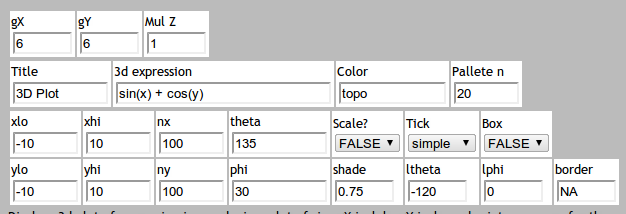
The part of the menu page for the settings of 3d plots is shown here:

Drawing quantile-quantile qq plots with R

Quantile-quantile plots gives the most visually appealing method to view the extent of normality of a vector or a two-column matrix of data. Data is either a single column (Y) or two column (X, Y). If nvars is 1, will display qqnorm(y). Otherwise, if nvars is 2, will display qqplot(x,y). Data is always read row wise(byrow=TRUE).

Optionally, line passing thru Q1 and Q3 is drawn if Line? is TRUE. If data on X axis is TRUE, data values will be shown in X-axis otherwise on the Y-axis.


A qq plot may be generated by our solver at /solvers/rplotpage/qq

Drawing quiver plots with R

Our extreme solvers site solvers/rplotpage/quiver
allows one to draw a quiver plot or arrows plot over a displayed image of a function in two variables of the form $$fxy= f(x,y)$$. It is based on R routines by Ripley and Hand and illustrated in the addictedtor.org gallery from which our qpy code is based.

Here is an example for the function (or expression) $$fxy= \sin(x) + \cos(y)$$. Here we have the settings xlo=ylo = -2.0, xhi=yhi=2.0 and xby=yby = 0.2. The contour color is gray and the pallette for the image is terrain.colors. Here is the output image.


Note that we have shown a test code to generate quiver plots previously.

Generating quiver plots using R under Python

Here is Python code to generate an R script which in turn does the actual image generation.

"""
quiver-test.py
"""

def quiverfunc(fxy, x0, x1, xby, y0, y1, yby, pallette="terrain.colors", contourcolor="gray"):
   S = """
par.uin <- function() 
  # determine scale of inches/userunits in x and y
  # from http://tolstoy.newcastle.edu.au/R/help/01c/2714.html
  # Brian Ripley Tue 20 Nov 2001 - 20:13:52 EST
 {
    u <- par("usr") 
    p <- par("pin") 
    c(p[1]/(u[2] - u[1]), p[2]/(u[4] - u[3]))
 }

quiver2 <- function(expr,
                     x,
                     y,
                     nlevels=20, 
                     length=0.05, 
                     ...){

    z <- expand.grid(x,y) 
    xx  <- x
    x   <- z[,1]
    yy  <- y
    y   <- z[,2]

    fxy <- eval(expr) 
    grad_x <- eval(D(expr, "x")) 
    grad_y <- eval(D(expr, "y")) 

  dim(fxy) <- c(length(xx), length(yy)) 
  dim(grad_x) <- dim(fxy) 
  dim(grad_y) <- dim(fxy) 

  maxlen <- min(diff(xx), diff(yy)) * .9 
  grad_x <- grad_x / max(grad_x) * maxlen 
  grad_y <- grad_y / max(grad_y) * maxlen 

  filled.contour(xx, yy, fxy, nlevels=nlevels, 
    plot.axes = { 
      contour(xx, yy, fxy, add=T, col="gray", 
              nlevels=nlevels, drawlabels=FALSE) 

      arrows(x0  = x, 
             x1  = x + grad_x,
             y0  = y,
             y1  = y + grad_y,
             length = length*min(par.uin())) 

      axis(1) 
      axis(2) 
    },
    ...)
}

f <- expression( #expr) 
x <- seq(#x0, #x1,by= #xby) 
y <- seq(#y0, #y1,by= #yby) 
par(mar=c(3,3,3,3)) 
quiver2(f,x,y, color.palette=#pallette) 
graphics.off()
"""
   S = S.replace("#expr", fxy)
   S = S.replace("#x0", x0)
   S = S.replace("#x1", x1)
   S = S.replace("#xby",xby)
   S = S.replace("#y0", y0)
   S = S.replace("#y1", y1)
   S = S.replace("#yby",yby)
   S = S.replace("#pallette",pallette)
   S = S.replace("#contourcol", contourcolor)
   return S 

Rcode = 'png("temp.png", 6 *72, 6 *72)'
Rcode +=  quiverfunc("(3*x^2 + y) * exp(-x^2-y^2)", "-2", "2", "0.2", "-2", "2", "0.2", pallette="terrain.colors", contourcolor="gray")
print Rcode
Save the file to "test-quiver2.py". Then to run it, type python quiver2.py > out.R. Then issue R < out.R --no-save. The generated image is in temp.png. Finally, display it using the imagemagick tool: display temp.png.

Sunday, August 22, 2010

Drawing pie plots with R

Pie plots are the most unadorned graphs in R. Those developers of R even warn of using pie plots for conveying information and instead recommend using a bar plot or dot chart.
Here is an example of a pie chart drawn using R.


In the page for pie chart generation, the radius of the pie is relative to the size of the graph and thus has a maximum value of 1.

Drawing polar plots in three ways using R

A polar plot relates r as a function of angle theta, $$\theta$$. The rectangular components can be
computed can be computed separately as $$x = r cos(theta)$$ and $$y = r sin(theta)$$.

Our solver page at http://extreme.adorio-research.org/solvers/rplotpage/polar/ has three different ways to present polar plots, namely
[polar, rectangular and space]. The range of theta can be specified and the number of points can be set up to 15000, to allow fast drawing without overloading the server.

Here are the three images possible for the butterfly equation, exp(cos(theta)) - 2 * cos(4*theta) + sin(theta/12)^5, presented in Venables and Ripley authoritative book: MASS "Modern Applied Statistics using S" book.


The last image was generated using ntheta = 15000 and pch=5.

Here is the page QP/QPY code for the polar plot page.

# pie.qpy
# 2006.09.02   0.0.1  first version
# 2006.09.20   0.0.2  split from pie,pie, dot page.
# 2010.08.23   0.0.3  third version.

__version__ = "0.0.3"
__date__    = "07.08.12"
__author__  = "eadorio@yahoo.com"
__title__   = "Polar plots using R"
__catalog__ = "POLAR-RPLOT-0127"
__url__     = "/solvers/rplotpage/polar/"
__author__  = "E.P. Adorio"


import time
import tempfile
import commands
import os

from   qp.fill.directory  import Directory
from   qp.fill.form       import Form, StringWidget, TextWidget,CheckboxWidget,SingleSelectWidget
from   qp.fill.css   import BASIC_FORM_CSS

from   qp.sites.extreme.lib.tmpfilesmanager import TmpFilesManager
from   qp.sites.extreme.lib.uicommon        import renderheader, renderfooter, processheader, processfooter
from   qp.pub.common                        import page
from   qp.sites.extreme.lib.checkinput      import checkInputs, getFormStrings
from   qp.sites.extreme.lib.qpyutils        import printRlines, showLogo
from   qp.sites.extreme.lib.webutils        import vecRead,GraphicsFile, as_R_cvector, as_R_vector, as_R_matrix, runRcode
from   qp.sites.extreme.lib import config


def Solve(fields):
    (gX, gY, theta0, theta1, ntheta, gtype, psize, equation, col, main, sub, xlab, ylab) = fields

    fname1    = GraphicsFile("png")
    barefile1 = fname1.split(str("/")) [-1]

    Rcode = "png('%s', width=%s*72, height=%s*72)\n" % (fname1, gX, gY)
    Rcode += """
theta  <- seq(%s, %s, len=%s)   
radius <- %s
x      <- radius * cos(theta)
y      <- radius * sin(theta)
""" % (theta0, theta1, ntheta, equation)

    if gtype == "polar":
       Rcode += """
plot(y, x, col="%s",type="l",
     main="%s",sub="%s",xlab="%s",ylab="%s", axes=FALSE)
"""    % (col, main, sub, xlab, ylab)
    elif gtype == "rect":
       Rcode += """
vlo = min(radius, x, y)
vhi = max(radius, x, y)
plot(theta, radius,  ylim=c(vlo, vhi), col="black",type="l", main="%s",sub="%s",xlab="%s",ylab="%s")
points(theta, x,  col="red",type="l")
points(theta, y,  col="blue",type="l")
""" % (main, sub, xlab, ylab)
    elif gtype == "3d":
       Rcode += """
library(scatterplot3d)
scatterplot3d(x, y, theta, highlight.3d=TRUE, col.axis="blue",
              col.grid="lightblue", main="Space Curve", pch=16, cex.symbols = %s)
""" % psize
    Rcode += """
graphics.off()
#img %s
""" % (barefile1)
    status, output = runRcode(Rcode)
    return output
    

class PolarplotPage(Directory):
    def get_exports(self):
        yield ('', 'index', 'PolarPlot', '')
           

    def index[html](self):
        form  = Form(enctype="multipart/form-data")  # enctype for file upload
        form.add(StringWidget,  name="gX",  title = "gX",  value="6", size=3)
        form.add(StringWidget,  name="gY", title = "gY", value="6",  size=3)

        form.add(StringWidget,  name="theta0",  title = "theta0", value = "0", size=5)
        form.add(StringWidget,  name="theta1",  title = "theta1", value = "24*pi", size=5)
        form.add(StringWidget,  name="ntheta",  title = "ntheta", value = "2000", size = 5)
        form.add(SingleSelectWidget,  name="gtype",   title = "Type",
                 value = "polar", options = [("polar", "polar"), ("rect", "rect"),("3d", "space")])
        form.add(StringWidget,  name="psize",  title = "Pt size", value = "0.2", size = 3)

        form.add(StringWidget,  name="equation",  title="Equation in theta r = f(theta)", 
                 value= "exp(cos(theta)) - 2 * cos(4*theta) + sin(theta/12)^5", size = 70)
        form.add(StringWidget,  name="col", title="Color", value="red", size=10)
        form.add(StringWidget,  name="main",  title="Main", value="Polar Plot", size=15)
        form.add(StringWidget,  name="sub",   title="Sub",  value="Example",  size = 15)
        form.add(StringWidget,  name="xlab",  title="xlab", value="X",     size=15)
        form.add(StringWidget,  name="ylab",  title="ylab", value="Y",   size=15)

        form.add_hidden("time",   value = time.time())
        form.add_submit("submit", "submit")

        def render [html] ():
            renderheader(__title__)

            """\
    
%s %s %s %s %s %s %s %s
""" % (form.get_widget("gX").render(), form.get_widget("gY").render(), form.get_widget("theta0").render(), form.get_widget("theta1").render(), form.get_widget("ntheta").render(), form.get_widget("gtype").render(), form.get_widget("col").render(), form.get_widget("psize").render(), ) """\
%s
""" % ( form.get_widget("equation").render(), ) """
%s %s %s %s
""" % (form.get_widget("main").render(), form.get_widget("sub").render(), form.get_widget("xlab").render(), form.get_widget("ylab").render(), ) """ Draws 2D polar plots r vs theta or rectangular plots (r,x,y vs theta) or 3D space curves (x,y,theta) for equation involving theta. The size of the plot is approximately gX inch by gY inch (limited to 10). The point in a space curve will be drawn using filled circles with size determined by Pt size. The following bounds apply to the Open Solver version:
gX float 3, 10
gY float 3, 10
ntheta int 2, 15000
psize float 0.2, 10

Space curves are drawn using the R scatterplot3d package of Uwe Ligges. The butterfly polar function example is from Venables and Ripley, MASS.
""" renderfooter(form, __version__, __catalog__, __author__) if not form.is_submitted(): return page('polarplotpage', render(), style= BASIC_FORM_CSS) def process [html] (): processheader(__title__) calctime_start = time.time() # Get the form input values def tmp1(): return getFormStrings(form, [ "gX", "gY", "theta0", "theta1", "ntheta", "gtype", "psize", "equation", "col", "main", "sub", "xlab", "ylab"]) (gX, gY, theta0, theta1, ntheta, gtype, psize, equation, col, main, sub, xlab, ylab) = tmp1() def tmp2(): inflag = checkInputs( [("gX", gX, ("float", 3, 10)), ("gY", gY, ("float", 3, 10)), ("theta0", theta0, ("eqn", "")), ("theta1", theta1, ("eqn", "")), ("ntheta", ntheta, ("int", 2, 15000)), ("psize", psize, ("float", 0.2, 10)), ("equation", equation, ("eqn",""))]) return inflag inflag = tmp2() if inflag[0]: "

"
               inflag[1]
               "
" else: output = Solve((gX, gY, theta0, theta1, ntheta, gtype, psize, equation, col, main, sub, xlab, ylab)) "
"
               printRlines(output)
               "
" showLogo("Rlogo.jpg") processfooter(form, calctime_start, "./", __url__) process()

Constructive criticisms from our reader are very welcome. Email the page author at ernesto.adorio@gmail.com or alternately at eadorio@yahoo.com

Installing R packages inside R itself.

I am reviewing all my solvers one at a time. The scatterplot page has an option to draw in theee dimensions! this is made possible by the scatterplot3d. Alas, when I clicked to generate the graph, the library was not there since we updated to the latest and greatest version 2.11.1 of R!

Ah ok. Assume you know the package name. Run R with root privileges, sudo R. then issue
install.packages ("scatterplot3d", repos="http://cran.r-project.org/") Then watch R do its intallation procedure.


> install.packages ("scatterplot3d", repos="http://cran.r-project.org/")
trying URL 'http://cran.r-project.org/src/contrib/scatterplot3d_0.3-30.tar.gz'
Content type 'application/x-gzip' length 508829 bytes (496 Kb)
opened URL
==================================================
downloaded 496 Kb


Test if the install was successful: library("scatterplot3d") There should be no error messages.

Drawing a matrix plot with R

Catalog MATRIX-RPLOT-0129
Version 0003
Date 08.23.10
URL /solvers/rplotpage/matrix
Source File /solvers/plots/rplot/matrix.qpy
Doc File /solvers/plots/rplot/doc/rplot.tex
XML-RPC TBD
Solvers Python, R
Author Dr. Ernesto P. Adorio


The matplot function of R allows the user to plot other vectors against a given vector.
Given an input matrix X, our matrix plot allows one to specify a "base" column for which the other
columns are plotted against it.

Various plot settings allows one to plot either points or lines for other columns.
The main input box expects a matrix with each row written on each line.
A maximum of seven columns is allowed by this matrix plot routine.

Here is a view of the matrix plot page menu screen:


And here is the resulting plot drawn by our online solver.


The actual R code to generate the graph is

png('tmpksstQF.png', width=6*72, height=6*72)
> X <- c(21.69935,-11.798573,104.36818,33.40331,-12.988921,105.79699,48.8454,-12.244453,111.39495,44.10297,-9.557104,136 15997,48.51514,-7.568557,150.82756,65.80403,-9.416977,147.99936,34.86882,-8.473734,93.32171,45.74425,-7.322524,83.93707, 1.8046,-4.894993,151.96477,54.41312,-5.934022,43.50714,53.41098,-10.627767,91.71084,58.93975,-11.212206,118.9405,35.4372 ,-8.715245,55.91096,56.1509,-13.563171,40.80423,81.91758,-11.491009,95.21836,42.168,-13.77088,100.34292,55.15041,-7.5223 7,68.27453,35.32567,-8.874406,129.32671,49.89936,-16.804003,112.49538,43.73633,-8.427571,47.67621,52.84546,-8.812953,88. 2893,55.83368,-10.618802,108.34818,37.9956,-11.34301,64.80144,47.22976,-14.296704,95.19047,62.69356,-11.104689,89.95547) > M <- matrix(X, ncol = 3, byrow=T) > M <- M[order(M[,1]),] > M
> matplot( M[,1], M[,-1],type=c('p','p','p','p','p','p'),lty=c(2,2,2,2,2,2),
+ lwd=c(1,1,1,1,1,1),pch=c(1,2,3,4,5,6),col=c('black','blue','red','green','yellow','violet'),
+ cex=c(1,1,1,1,1,1),ylab=c('y,z'),xlab=c('x'),main="Matrix plot",sub="matplot generator")
> graphics.off()
> #img tmpksstQF.png

The Qpy code is presented here so that improvements may be facilitated faster.
# matrix.qpy
# 2006.09.02   0.0.1  first version
# 2006.09.20   0.0.2  split from pie, dot page.
# 2010.08.23   0.0.3  revised.


__version__ = "0.0.3 2010.08.23"
__author__  = "ernesto.adorio@gmail.com"
__title__   = "Matrix PLots using R"
__catalog__ = "MATPLOT-RPLOT-0129"
__url__     = "/solvers/rplotpage/matrix/"


import time
import tempfile
import commands
import os

from   qp.fill.directory  import Directory
from   qp.fill.form       import Form, StringWidget, TextWidget,CheckboxWidget,SingleSelectWidget
from   qp.fill.css   import BASIC_FORM_CSS

from   qp.sites.extreme.lib.tmpfilesmanager import TmpFilesManager
from   qp.sites.extreme.lib.uicommon        import renderheader, renderfooter, processheader, processfooter
from   qp.pub.common                        import page
from   qp.sites.extreme.lib.checkinput      import checkInputs, getFormStrings
from   qp.sites.extreme.lib.qpyutils        import printRlines, showLogo
from   qp.sites.extreme.lib.webutils        import vecRead, GraphicsFile, as_R_cvector, as_R_vector, as_R_matrix
from   qp.sites.extreme.lib import config


def getcarg(s, defaultval):
    s = s.strip()
    if s in ["", "None"]:
       return defaultval
    return as_R_cvector(s.split())
   

def getdarg(s, defaultval):
    s = s.strip()
    if s in ["", "None"]:
       return defaultval
    return as_R_vector(s.split())
   
def Solve(fields):
    # Get the fields.
    (gX, gY, matdata, colnames, against, sortq, plottype, lty, lwd, pch, cex, xlab, ylab, col,main, sub) = fields

    if colnames == "": return "ERROR: blank column names field"
    colnames = colnames.split()

    ncol     = len(colnames)
    if ncol > 7:
       return "ERROR: more than 7 columns specified."

    against = against.strip()     
    if against not in ["None",""]:
       try:
           apos = colnames.index(against) + 1
       except:
           raise ValueError, "Variable to plot against [%s]is not in column names." % against
    else:
       apos = 0

    matdata=matdata.strip() 
    if matdata in ["", "None"]: 
       raise ValueError, "ERROR: empty matrix data field."   
    X = vecRead(matdata)

    extraargs = ""
    extraargs += ',type=%s' % getcarg(plottype, "p")
    extraargs += ',lty=%s'   % getdarg(lty, 1)
    extraargs += ',lwd=%s'   % getdarg(lwd, 1)
    extraargs += ',pch=%s'   % getdarg(pch, "c(1,2,3,4,5,6,7)")
    extraargs += ',col=%s'   % getcarg(col, "black")
    extraargs += ',cex=%s'   % getdarg(cex, 1)
    extraargs += ',ylab=%s'  % getcarg(ylab, '""')
    extraargs += ',xlab=%s' % getcarg(xlab, '""')
    extraargs += ',main="%s"'  % main
    extraargs += ',sub="%s"'  % sub


    # Start of R code.
    fname1    = GraphicsFile(str("png"))
    barefile1 = fname1.split(str("/"))[-1]
    Rcode = """png('%s', width=6*72, height=6*72)\n""" % fname1
    Rcode += "X <- " + as_R_vector(X) + "\n"
    Rcode += """M <- matrix(X, ncol = %s, byrow=T)\n""" % ncol
    if apos != 0:
        if sortq:
           Rcode += "M <- M[order(M[,%s]),]\n" % apos
        Rcode += "M\n"
        Rcode += "matplot( M[,%s], M[,-%s] %s)" %(apos,apos, extraargs)
    else:
        Rcode += "matplot(M %s)" % extraargs

    Rcode += """
graphics.off()
#img %s
    """ % (barefile1,)

    # Write to temporary file.
    (f, name) = tempfile.mkstemp(suffix=str(".r"), prefix=str("tmp"), dir=config.tmp_dir)
    os.write(f, str(Rcode))
    (status, output) = commands.getstatusoutput(str("R -q --no-save < %s")  % name)
    os.close(f)  
    return output
    

class MatrixplotPage(Directory):
    def get_exports(self):
        yield ('', 'index', 'MatrixPlot', '')
           

    def index[html](self):
        form  = Form(enctype="multipart/form-data")  # enctype for file upload
        form.add(StringWidget, name="gX", title="gX", value = "6", size=3)
        form.add(StringWidget, name="gY", title="gY", value = "6", size=3)

        sample = """
    21.69935 -11.798573 104.36818
    33.40331 -12.988921 105.79699
    48.84540 -12.244453 111.39495
    44.10297  -9.557104 136.15997
    48.51514  -7.568557 150.82756
    65.80403  -9.416977 147.99936
    34.86882  -8.473734  93.32171
    45.74425  -7.322524  83.93707
    71.80460  -4.894993 151.96477
    54.41312  -5.934022  43.50714
    53.41098 -10.627767  91.71084
    58.93975 -11.212206 118.94050
    35.43727  -8.715245  55.91096
    56.15090 -13.563171  40.80423
    81.91758 -11.491009  95.21836
    42.16800 -13.770880 100.34292
    55.15041  -7.522367  68.27453
    35.32567  -8.874406 129.32671
    49.89936 -16.804003 112.49538
    43.73633  -8.427571  47.67621
    52.84546  -8.812953  88.02893
    55.83368 -10.618802 108.34818
    37.99560 -11.343010  64.80144
    47.22976 -14.296704  95.19047
    62.69356 -11.104689  89.95547
    """
        form.add(TextWidget,    name = "matdata", title="", \
                 value = sample, cols ="65", rows = "10")

        form.add(StringWidget,  name = "colnames", title="Column names (not blank!)",
                 value = "x y z", size = "35")

        form.add(StringWidget,  name = "against", title="Against", value = "x", size = "10")
        form.add(CheckboxWidget, name = "sortq",   title="Sort?")

        form.add(StringWidget,  name = "plottype", size = 35, value = "p p p p p p")
        form.add(StringWidget,  name = "lty",      size = 35, value = "2 2 2 2 2 2")
        form.add(StringWidget,  name = "lwd",      size = 35, value = "1 1 1 1 1 1")
        form.add(StringWidget,  name = "pch",      size = 35, value = "1 2 3 4 5 6")
        form.add(StringWidget,  name = "cex",      size = 35, value = "1 1 1 1 1 1")
        form.add(StringWidget,  name = "xlab",     size = 35, value = "x")
        form.add(StringWidget,  name = "ylab",     size = 35, value = "y,z")
        form.add(StringWidget,  name = "main",     size = 35, value = "Matrix plot")
        form.add(StringWidget,  name = "sub",      size = 35, value = "matplot generator")
        form.add(StringWidget,  name = "col",      size = 35, value = "black blue red green yellow violet")

        form.add_hidden("time",   value = time.time())
        form.add_submit("submit", "submit")

        def render [html] ():
            renderheader(__title__)

            """
            
%s%s%s%s%s
""" % (form.get_widget("gX").render(), form.get_widget("gY").render(), form.get_widget("colnames").render(), form.get_widget("against").render(), form.get_widget("sortq").render(), ) form.get_widget("matdata").render() """
Plot type, type [p l b c o h s S n] %s
Line type, lty [1 2 3 4 5] %s
Line width, lwd %s
Point char, pch [any character]] %s
Char expand, cex %s
X label, xlab %s
Y label, ylab %s
Colors, col %s
Main title, main %s
Subtitle, sub %s
""" % (form.get_widget("plottype").render(), form.get_widget("lty").render(), form.get_widget("lwd").render(), form.get_widget("pch").render(), form.get_widget("cex").render(), form.get_widget("xlab").render(), form.get_widget("ylab").render(), form.get_widget("col").render(), form.get_widget("main").render(), form.get_widget("sub").render()) """ Uses matplot() function of R to plot up to 7 columns of data. The image size is gX inch by gY inch. Use can specify various graphics parameters such as colors, plotting character and labels. Up to six columns can be plotted. When plotting against a specified column, it may be important to sort the matrix based on the specified column if plotting using lines.

When statistics, pairs plots and box blots are required, use the solver Cat STAT-MSS-0064 instead. """ renderfooter(form, __version__, __catalog__, __author__) if not form.is_submitted(): return page('matrixplotpage', render(), style= BASIC_FORM_CSS) def process [html] (): processheader(__title__) calctime_start = time.time() # Get the problem parameters (gX, gY, matdata, colnames, against, sortq, plottype, lty, lwd, pch, cex, xlab, ylab, col, main, sub) = getFormStrings(form, [ "gX", "gY", "matdata", "colnames", "against", "sortq","plottype", "lty", "lwd", "pch", "cex", "xlab", "ylab", "col", "main", "sub" ]) inflag = checkInputs( [("gX", gX, ("float", 3, 10)), ("gY", gY, ("float", 3, 10)), ]) if inflag[0]: "

"
               inflag[1]
               "
" else: output = Solve((gX, gY, matdata, colnames, against, sortq, plottype, lty, lwd, pch, cex, xlab, ylab, col, main, sub)) "
"
               printRlines(output)
               "
" showLogo("Rlogo.jpg") processfooter(form, calctime_start, "./", __url__) process()

Constructive comments from our blog readers are always welcome.

Drawing a dotchart for dataframe in R

It has been suggested that bar charts and dot plots are excellent for displaying grouped data.
The dotchart function in R has the following syntax(typing ?dotchart inside an R session):


Cleveland's Dot Plots

Description:

Draw a Cleveland dot plot.

Usage:

dotchart(x, labels = NULL, groups = NULL, gdata = NULL,
cex = par("cex"), pch = 21, gpch = 21, bg = par("bg"),
color = par("fg"), gcolor = par("fg"), lcolor = "gray",
xlim = range(x[is.finite(x)]),
main = NULL, xlab = NULL, ylab = NULL, ...)

Arguments:

x: either a vector or matrix of numeric values (‘NA’s are
allowed). If ‘x’ is a matrix the overall plot consists of
juxtaposed dotplots for each row.

labels: a vector of labels for each point. For vectors the default
is to use ‘names(x)’ and for matrices the row labels
‘dimnames(x)[[1]]’.

..... More! please read the rest from an actual R session.


If R is a dataframe with column names (header) and row names, then the dot chart will use these
labels to group the data. Each column of data constitute a group and for each group, a series of
dot charts are displayed for all the rows belonging to the group.

Surprisingly, R does not display a dataframe natively inspite of the builtin VADeaths dataset working. Copying the VADeaths dataset to a file and reading it as a dataframe, (replacing embedded spaces with an underscore), resulted in R giving an error message that it expects a matrix or vector(roughly, a one column matrix). So we typecast it as a matrix and we are able to use the dotchart function.

Here is the menu page of our dotchart generator:


and a sample output.


We hasten to add that our page for a dot chart generator is only for quick visualization of data.

Syntax highlighter problems.

The new?? version of Alex Gorbatchev Syntax Highlighter when installed in our extreme-solvers.blogspot blog does not allow source code view, or copyging to the clipboard, or even rapid printing.

We will check if something is amiss in our installation.